Impulse Response Function
So far, we have considered a single neuron together with its receptive field. We now consider the case where the retina projects to an entire layer of neurons with identical but space-shifted receptive fields.
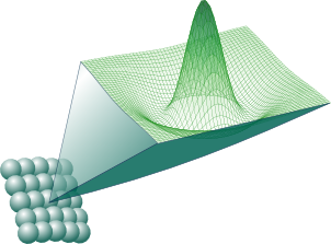
Layer of neurons with identical receptive fields.
If a point stimulus is delivered to this layer and we measure how this affects the activity of the cells in the layer, we will get a distribution of activity denoted as \( R ( \mathbf{r}_{c} ) \), where \( \mathbf{r}_{c} \) is the location of a neuron and \( R(\mathbf{r}_{c}) \) its activity. For general images composed of many point stimuli, we obtain:
\begin{equation} R(x_{c}, y_{c}) = R_{0} +\displaystyle\sum_i\sum_jW(x_{c} - x_i,y_{c} - y_j) S(x_i, y_j), \end{equation}
or, in the infinitesimal formulation
\begin{equation} R(\mathbf{r}_{c}) = R_{0} +\displaystyle \iint_\mathbf{r} W(\mathbf{r}_{c} - \mathbf{r}) S(\mathbf{r}) \; \mathrm{d}^2\mathbf{r}, \end{equation}
where \( R_{0} \) is the background firing rate and \(W\) is the weighting function describing the strength, or weight, with which a stimulus delivered at retinal position \(\mathbf{r}\) influences the output at \( \mathbf{r}_{c} \).
The weighting function can in principle be obtained by measuring the response to briefly flicking test spots positioned at different positions \(\mathbf{r}_\mathrm{s}\) which are very small (\(\sim \delta(\mathbf{r} - \mathbf{r}_\mathrm{s})\)) [1]. Mathematically this corresponds to a stimulus function given by
\begin{equation} S(\mathbf{r}, t) = L_s \delta(\mathbf{r} - \mathbf{r}_s), \end{equation}
where \(L_s\) is the luminance of the test spot. Inserting this into the equation we obtain the response (assuming zero background firing)
\begin{equation} R(\mathbf{r}_{c}) = L_s W(\mathbf{r}_{c} - \mathbf{r}_s). \end{equation}
The weighting function is thus in principle given by the measured firing rates of identical neurons located at various positions \(\mathbf{r}_{c} \) in the visual field following a \( \delta \)-pulse at position \( \mathbf{r}_s \). Because of this interpretation, the weighting factor is often referred to as the impulse-response function.
Relation to receptive field function
Assuming again a uniform layer of neurons with identical but space-shifted receptive fields, we obtain that a neuron at location \((x_{c}, y_{c}) \) will have a receptive field function \(F(\mathbf{r}-\mathbf{r}_{c} ) \). The response can then be written as
\begin{equation} R(\mathbf{r}_{c}) = R_{0} +\displaystyle \iint_\mathbf{r} F(\mathbf{r}- \mathbf{r}_{c} ) S(\mathbf{r}) \; \mathrm{d}^2\mathbf{r}. \end{equation}
By comparing this with the corrosponding equation expressed in terms of the impulse response function for all possible stimulus \(S \), we find that
\begin{equation} F(\mathbf{r}) = W(-\mathbf{r}), \end{equation}
i.e. the impulse response function and the receptive field function are mirrored versions of each other, for translation-invariant systems [2].
References
[1] Einevoll, Gaute T., and Hans E. Plesser. "Extended difference-of-Gaussians model incorporating cortical feedback for relay cells in the lateral geniculate nucleus of cat." Cognitive neurodynamics 6.4 (2012): 307-324.
[2] Mallot HA. Computational neuroscience: A First Course. vol. 9; 2013.